Vision Transformer

Vision-Transformer

Paper: https://arxiv.org/pdf/2010.11929.pdf

Transformer의 설명:

• https://jalammar.github.io/illustrated-transformer/
• https://github.com/FrancescoSaverioZuppichini/ViT
• https://github.com/jeonsworld/ViT-pytorch : reproduction이 거의 된 repo

Useful Video :

An Image is Worth 16x16 Words: Transformers for Image Recognition at Scale (Paper Explained)

Image vs NLP

To many pixels in images : It makes computer to process through transformer encoder. 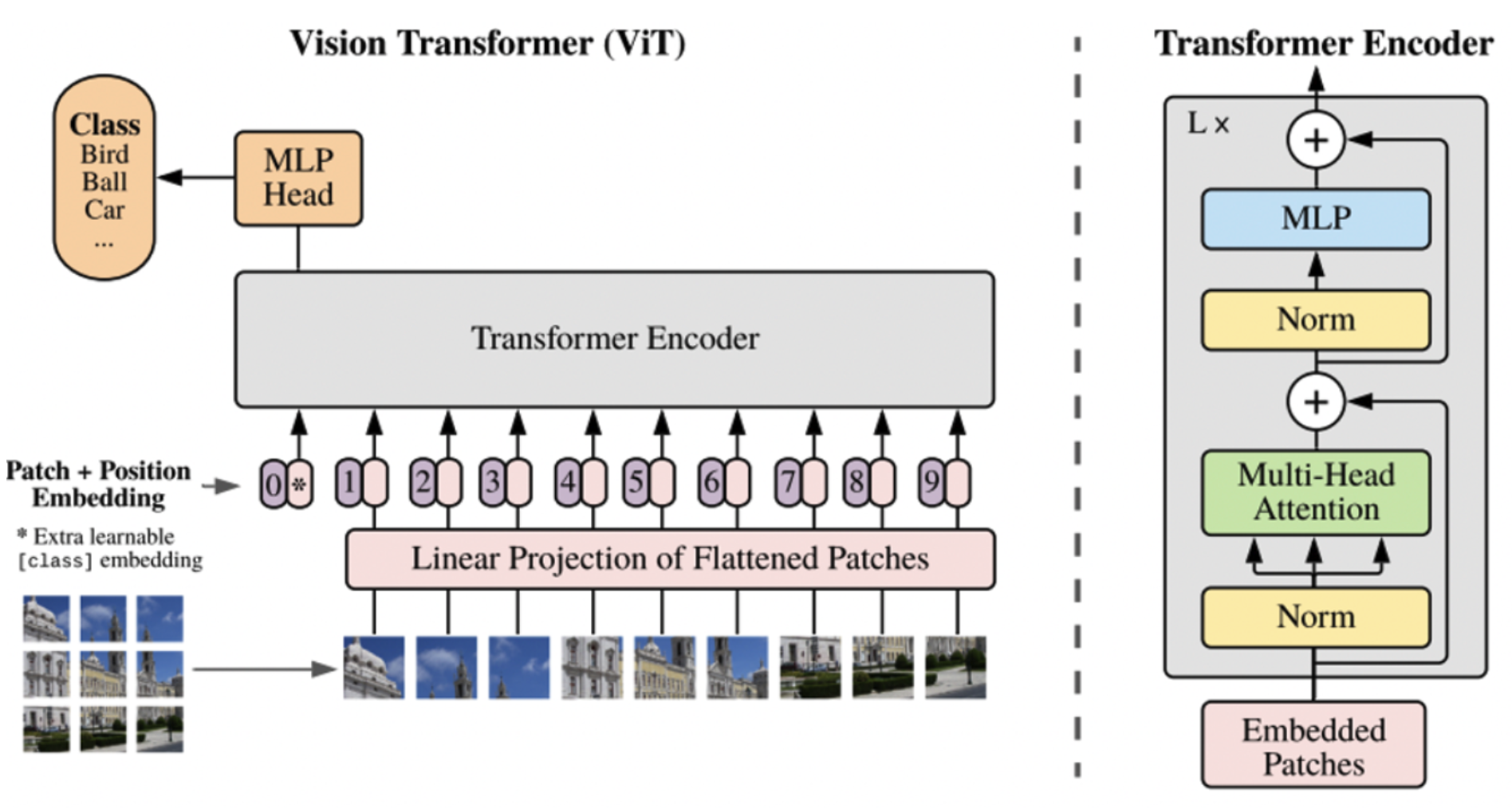## Introduction of Architecture

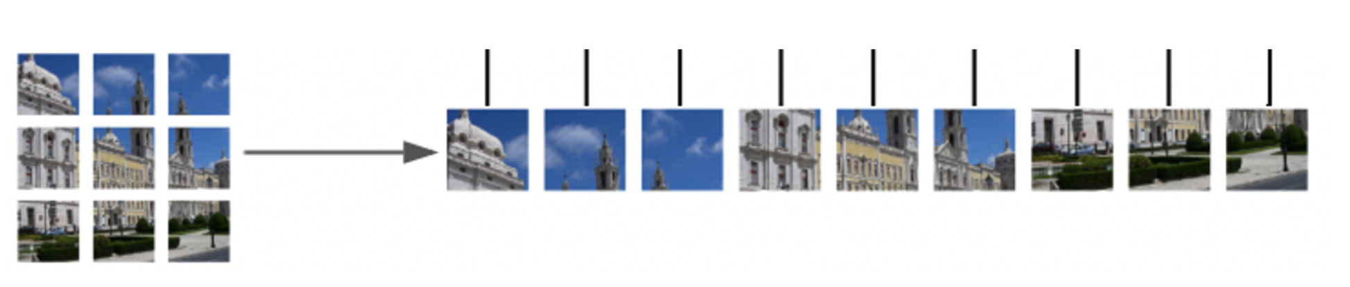
Patches

이미지를 16x16사이즈의 패치로 자름

Positional Embedding

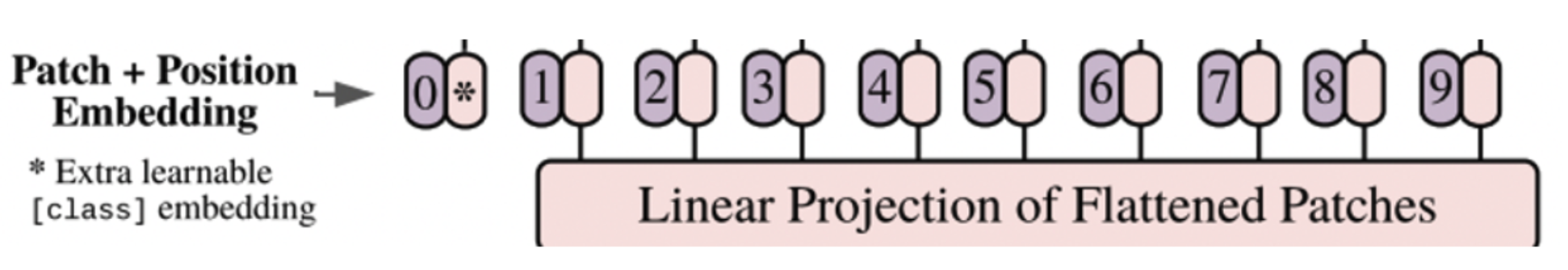- Learnable Positional embedding - 각 이미지 패치가 어느 위치인지 정해줌 - Positional embedding vector : Patch 를 vector로 변환한 후, E라는 positional embedding matrix에 곱해줌. (결국 fcn연산과 같음)

Transformer Encoder

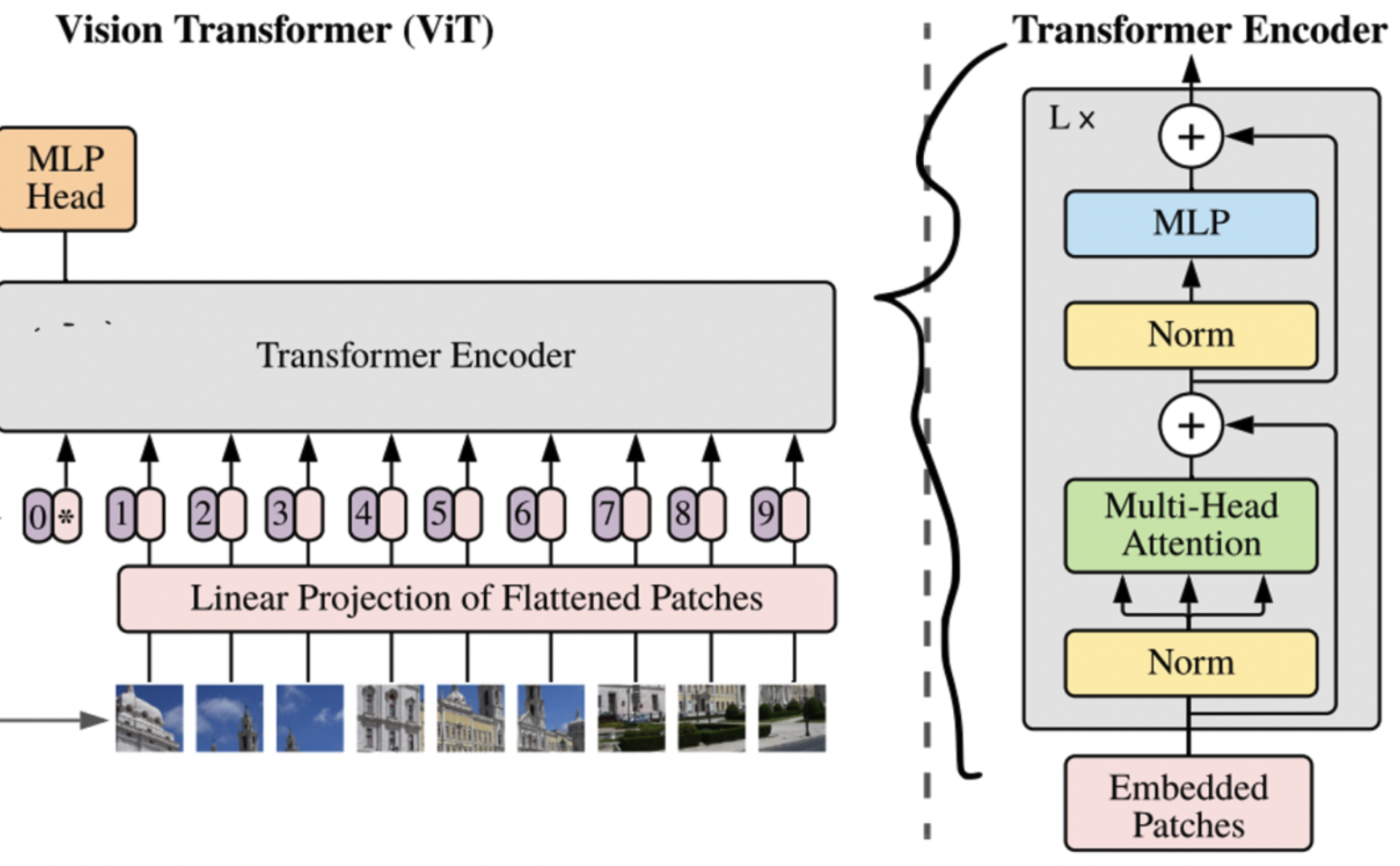
• Encoder layer를 거쳐 output출력을 위한 feature를 뽑아냄.
• Norm_first: True
  • layer norm is dnoe prior to attention and feedforward operations.

Classification Header

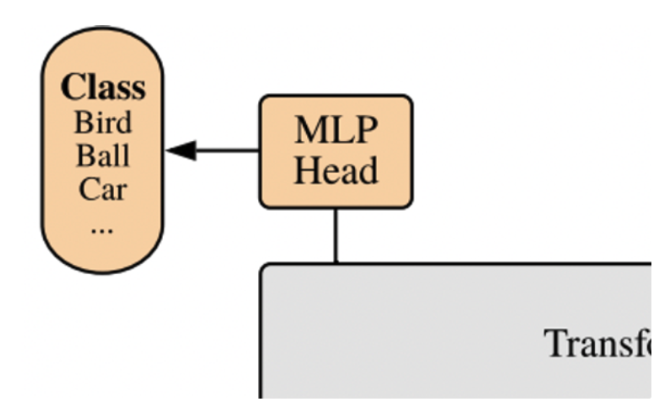- Multi-layer perceptron for classification

구현

einops 라이브러리를 설치하자

Tutorial 참고 https://github.com/arogozhnikov/einops, 쓸만할듯하니 자주 이용할듯

pip install einops

Import Required Packages

import torch
import torch.nn.functional as F
import matplotlib.pyplot as plt

from torch import nn
from torch import Tensor
from PIL import Image
from torchvision.transforms import Compose, Resize, ToTensor
from einops import rearrange, reduce, repeat
from einops.layers.torch import Rearrange, Reduce
from torchsummary import summary

Data Loader

아래는 ipython예시

Vision-Transformer/transformer_patch.ipynb at master · jonggyujang0123/Vision-Transformer

First, download a cat image

wget [<https://github.com/FrancescoSaverioZuppichini/ViT/blob/main/cat.jpg>](<https://raw.githubusercontent.com/FrancescoSaverioZuppichini/ViT/main/cat.jpg>)

Patch

from PIL import Image
import numpy as np 
import matplotlib.pyplot as plt
from torchvision.transforms import Compose, Resize, ToTensor
from einops import rearrange, reduce, repeat

img = Image.open('../cat.jpg')

fig = plt.figure()
plt.imshow(img)

patch_size = 16 # 16 pixels
pathes = rearrange(x, 'b c (h s1) (w s2) -> b (h w) (s1 s2 c)', s1=patch_size, s2=patch_size)
print(pathes.size())

# plt.imshow(rearrange(pathes, 'b (i1 i2) (h w c) -> (i1 h) (i2 w) (b c)', h = 16, w=16, i1=14, i2=14))

plt.title('100-path patch is : ')
plt.imshow(rearrange(pathes[:,100,:], 'b (h w c) -> h w (b c)', h = 16, w=16))

patch_size = 16 # 16 pixels
pathes = rearrange(x, 'b c (h s1) (w s2) -> b (h w) (s1 s2 c)', s1=patch_size, s2=patch_size)
print(pathes.size())

# plt.imshow(rearrange(pathes, 'b (i1 i2) (h w c) -> (i1 h) (i2 w) (b c)', h = 16, w=16, i1=14, i2=14))

plt.title('100-path patch is : ')
plt.imshow(rearrange(pathes[:,100,:], 'b (h w c) -> h w (b c)', h = 16, w=16))33

Patch embedding

• 16x16으로 잘라낸 패치들 (각 768개의 feature를 가지고 있음) 을 nn.Linear를 통해 embedding시킴.
• input : image (1, 3, 224, 224) [b c h w]
• output : embedding vector (1, 196, 768) [b, patch, embed_feature]

class PatchEmbedding(nn.Module):
    def __init__(self, in_channels: int = 3, patch_size: int = 16, emb_size: int = 768):
        self.patch_size = patch_size
        super().__init__()
        self.projection = nn.Sequential(
            # using a conv layer instead of a linear one -> performance gains
            nn.Conv2d(in_channels, emb_size, kernel_size=patch_size, stride=patch_size),
            Rearrange('b e (h) (w) -> b (h w) e'),
        )
                
    def forward(self, x: Tensor) -> Tensor:
        x = self.projection(x)
        return x
    
PatchEmbedding()(x).shape

Cls (Classification) Token

• Cls token이란, embedding vector(768 길이)의 sequence맨앞에 임의의 768길이의 벡터를 붙임.
• 예를들면 [cls] [patch 0] [patch 1] … 이런식이됨.
• Segment embd와 position embd 가 항상 고정된 벡터이고 특징으로써는 의미가 없음.
• Encoder에서 이 token에 다른 patch들의 정보를 인코딩한다는 것은 전체 sequence의 정보를 담는 것과 같음.
• it is an aggregate representation of the sequence.
• 마지막에 transformer encoder를 거친 cls token 위치의 벡터를 가지고 classification을 함.
• 왜 필요하냐?
  • 첫번째 패치의 위치에 대해 수행하게 되면, 그 패치의 feature가 유독 강조되기 때문에 cls token이 필요함.
• 첫번째 위치에 concatenate함

class PatchEmbedding(nn.Module):
    def __init__(self, in_channels: int = 3, patch_size: int = 16, emb_size: int = 768):
        self.patch_size = patch_size
        super().__init__()
        self.projection = nn.Sequential(
            # using a conv layer instead of a linear one -> performance gains
            nn.Conv2d(in_channels, emb_size, kernel_size=patch_size, stride=patch_size),
            Rearrange('b e (h) (w) -> b (h w) e'),
        )
        
        self.cls_token = nn.Parameter(torch.randn(1,1, emb_size))
        
    def forward(self, x: Tensor) -> Tensor:
        b, _, _, _ = x.shape
        x = self.projection(x)
        cls_tokens = repeat(self.cls_token, '() n e -> b n e', b=b)
        # prepend the cls token to the input
        x = torch.cat([cls_tokens, x], dim=1)
        return x
    
PatchEmbedding()(x).shape

Position Embedding

• 각 patch의 위치를 나타내기 위해 추가하는 임베딩임.
• 패치의 수 (img_size // patch_size )**2 + 하나의 cls벡터에 대한 position
• NLP에서하던것과 달리 learnable parameter를 설정함 (!!)
• concat이 아니라 그냥 더해주면 됨.

class PatchEmbedding(nn.Module):
    def __init__(self, in_channels: int = 3, patch_size: int = 16, emb_size: int = 768, img_size: int = 224):
        self.patch_size = patch_size
        super().__init__()
        self.projection = nn.Sequential(
            # using a conv layer instead of a linear one -> performance gains
            nn.Conv2d(in_channels, emb_size, kernel_size=patch_size, stride=patch_size),
            Rearrange('b e (h) (w) -> b (h w) e'),
        )
        self.cls_token = nn.Parameter(torch.randn(1,1, emb_size))
        self.positions = nn.Parameter(torch.randn((img_size // patch_size) **2 + 1, emb_size))

        
    def forward(self, x: Tensor) -> Tensor:
        b, _, _, _ = x.shape
        x = self.projection(x)
        cls_tokens = repeat(self.cls_token, '() n e -> b n e', b=b)
        # prepend the cls token to the input
        x = torch.cat([cls_tokens, x], dim=1)
        # add position embedding
        x += self.positions
        return x
    
PatchEmbedding()(x).shape

Transformer

Multihead Attention layer

Untitled

• 각 patch에 대한 embedding vector로 부터 query, key, value를 연산함.
  • embed_vec → Linear → query [1, 197, 768].
  • embed_vec → Linear → key [1, 197, 768].
  • embed_vec → Linear → value [1, 197, 768].
• Multi-head split
  • query, key, value 벡터를 각각 n_head (8)개의 벡터로 나눔.
  • 여기서 embedding vector 의 사이즈는 n_head의 배수가 되어야함.
• query와 key로부터 attention score를 연산함.
  • attention score : [batch, num_heads, query_len, key_len]
  • 여기서 query_len = key_len = patch의 수
• key_len에 대해 softmax를 취해 각 key마다 weight를 구함.
• sqrt(d) —> scailing factor (normalization)을 위함.
• Attention score [batch, num_heads, query_len, key_len] 를 value [batch, num_heads, query_len, embedding_size//8] 에 곱해서 weighted value 를 구함
• 마지막으로, 2번째 dim (head) 과 4번째 dim (embed)를 합쳐서 다음의 output을 만듬.
  • [batch, query_len, embedding_size]
• 마지막으로 projection을 통해 output을 구함.

class MultiHeadAttention(nn.Module):
    def __init__(self, emb_size: int = 768, num_heads: int = 8, dropout: float = 0):
        super().__init__()
        self.emb_size = emb_size
        self.num_heads = num_heads
        # fuse the queries, keys and values in one matrix
        self.qkv = nn.Linear(emb_size, emb_size * 3)
        self.att_drop = nn.Dropout(dropout)
        self.projection = nn.Linear(emb_size, emb_size)
        
    def forward(self, x : Tensor, mask: Tensor = None) -> Tensor:
        # split keys, queries and values in num_heads
        qkv = rearrange(self.qkv(x), "b n (h d qkv) -> (qkv) b h n d", h=self.num_heads, qkv=3)
        queries, keys, values = qkv[0], qkv[1], qkv[2]
        # sum up over the last axis
        energy = torch.einsum('bhqd, bhkd -> bhqk', queries, keys) # batch, num_heads, query_len, key_len
        if mask is not None:
            fill_value = torch.finfo(torch.float32).min
            energy.mask_fill(~mask, fill_value)
            
        scaling = self.emb_size ** (1/2)
        att = F.softmax(energy, dim=-1) / scaling
        att = self.att_drop(att)
        # sum up over the third axis
        out = torch.einsum('bhal, bhlv -> bhav ', att, values)
        out = rearrange(out, "b h n d -> b n (h d)")
        out = self.projection(out)
        return out
    
patches_embedded = PatchEmbedding()(x)
MultiHeadAttention()(patches_embedded).shape

Multi-layer perceptron (MLP) block

스크린샷 2022-07-25 오후 1.53.12.png

• MLP layer with 1 hidden layer (size of which is 4*emb_size)
  • Linear : emb_size → 4*emb_size
  • GELU (Gaussian Error Linear Unit)

    • if \(x\) is the input and \(X\sim N(0,1)\), we have \(\Phi(x)= P(X\le x)\).

    • \(\text{GELU}(x) = xP(x\le X) = x\Phi(x) = x\cdot 1/2 * [1+erf(x/\sqrt{2})]\)

      

      스크린샷 2022-07-25 오후 2.00.15.png

    • A smoothen version of the ReLU

  • Dropout
  • Linear: 4*emb_size → emb_size

class FeedForwardBlock(nn.Sequential):
    def __init__(self, emb_size: int, expansion: int = 4, drop_p: float = 0.):
        super().__init__(
            nn.Linear(emb_size, expansion * emb_size),
            nn.GELU(),
            nn.Dropout(drop_p),
            nn.Linear(expansion * emb_size, emb_size),
        )

Residual Block

• fn : x + fn(x)를 할건데, fn가 무엇인지 input으로 받음.
• fn 1 (self-attention block):
  • nn.LayerNorm
  • MultiHeadAttention
  • nn.Dropout
• fn 2 (feed-forward block):
  • nn.LayerNorm()
  • FeedForwardBlock()
  • nn.Dropout

class ResidualAdd(nn.Module):
    def __init__(self, fn):
        super().__init__()
        self.fn = fn
        
    def forward(self, x, **kwargs):
        res = x
        x = self.fn(x, **kwargs)
        x += res
        return xc

Transformer Encoder Block

• 하나의 encoder block을 생성함.

class TransformerEncoderBlock(nn.Sequential):
    def __init__(self,
                 emb_size: int = 768,
                 drop_p: float = 0.,
                 forward_expansion: int = 4,
                 forward_drop_p: float = 0.,
                 ** kwargs):
        super().__init__(
            ResidualAdd(nn.Sequential(
                nn.LayerNorm(emb_size),
                MultiHeadAttention(emb_size, **kwargs),
                nn.Dropout(drop_p)
            )),
            ResidualAdd(nn.Sequential(
                nn.LayerNorm(emb_size),
                FeedForwardBlock(
                    emb_size, expansion=forward_expansion, drop_p=forward_drop_p),
                nn.Dropout(drop_p)
            )
            ))

TransformerEncoder ( N layers)

• TransformerEncoderBlock을 쌓음.

class TransformerEncoder(nn.Sequential):
    def __init__(self, depth: int = 12, **kwargs):
        super().__init__(*[TransformerEncoderBlock(**kwargs) for _ in range(depth)])

Head Layer

• If classifier == token:
  • token에 해당하는 feature만 뽑아냄.
• If classifier == gap
  • token빼고 average취함.

class ClassificationHead(nn.Sequential):
    def __init__(self, emb_size: int = 768, n_classes: int = 1000):
                super().__init__(
                    Reduce('b n e -> b e', reduction='mean'),
                    nn.LayerNorm(emb_size), 
                    nn.Linear(emb_size, n_classes))

Vision Transformer (ViT) model

• Todo
  • ResNet 적용 (앞단에) 이 가능하게 고쳐야함.
  • classifier option 추가.
  • 데이터셋 추가하기
    • CIFAR-100 데이터
    • ImageNet 2012

class ViT(nn.Sequential):
    def __init__(self, in_channels=3, patch_size=16, emb_size=768, img_size=224, depth=12, n_classes=10, **kwargs):
        super().__init__(
            PatchEmbedding(in_channels, patch_size, emb_size, img_size),
            TransformerEncoder(depth, emb_size=emb_size, **kwargs),
            ClassificationHead(emb_size, n_classes)
        )

patches_embedded = PatchEmbedding()(x)
TransformerEncoderBlock()(patches_embedded).shape

# Result: torch.Size([1, 197, 768])

Simulation

# define the loss function, optimizer and lr_scheduler
loss_func = nn.CrossEntropyLoss(reduction='sum')
opt = optim.Adam(model.parameters(), lr=0.01)

from torch.optim.lr_scheduler import ReduceLROnPlateau
lr_scheduler = ReduceLROnPlateau(opt, mode='min', factor=0.1, patience=10)

시뮬레이션 목표

위에 까지만 정리하고 디테일한 코드는 vim으로 다시 작성하여 실행하고자 함.

위 설명과 다른점들 :

• ResNet 적용 (앞단에) 이 가능하게 고쳐야함.

• classifier option 추가.

• 데이터셋 추가하기

  • CIFAR-100 데이터
  • ImageNet 2012

• In particular, the best model reaches the accuracy of 88.55% on ImageNet, 90.72% on ImageNet-ReaL, 94.55% on CIFAR-100, and 77.63% on the VTAB suite of 19 tasks.